双摆的数值计算(Matlab)
贡献者: addis
- 本文处于草稿阶段。

图 1:双摆的运行结果,蓝色曲线显示末端的轨迹。动画见这里。
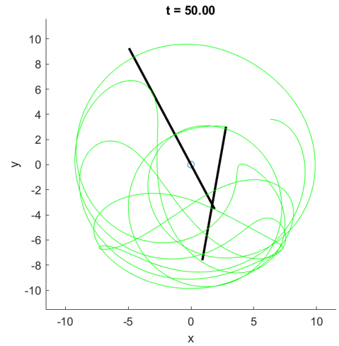
图 2:刚体双摆的运行结果,蓝色曲线显示末端的轨迹。动画见这里。

图 3:图 2 的模拟是对照电影《钢铁侠 2》中的摆件制作的。
未完成:添加摩擦力
代码 1:double_pendulum.m
% 双摆运动
function double_pendulum
% === 参数设置 ===
m1 = 1; l1 = 1; % 摆 1
m2 = 1; l2 = 1; % 摆 2
th10 = pi; th20 = pi; % 初始角度
w10 = -4; w20 = 6; % 初始角速度
g = 9.8; % 重力加速度
tmin = 0; tmax = 10; Nt = 200; % 时间网格
Nsmooth = 4; % 轨迹平滑(每两帧之间轨迹的线段数)
RelTol = 1e-6; % 微分方程精度
% ==============
close all;
Y0 = [th10; th20; w10; w20];
options = odeset('RelTol',RelTol);
[T, Y] = ode45(@(t,Y)odefun(t, Y, m1, m2, l1, l2, g), ...
        [tmin,tmax], Y0, options);
Th1 = Y(:,1); Th2 = Y(:,2); W1 = Y(:,3); W2 = Y(:,4);
Ek = 0.5*m1*(l1*W1).^2 + 0.5*m2*((l1*W1.*cos(Th1)+l2*W2.*cos(Th2)).^2 ...
    + (l1*W1.*sin(Th1) + l2*W2.*sin(Th2)).^2);
V = -m1*g*l1*cos(Th1) - m2*g*(l1*cos(Th1) + l2*cos(Th2));
figure; plot(T, Ek + V); xlabel time; title 'total energy';
t = linspace(tmin, tmax, Nt);
tt = linspace(tmin, tmax, Nsmooth*(Nt-1)+1);
th1 = interp1(T, Th1, t, 'spline');
thth1 = interp1(T, Th1, tt, 'spline');
th2 = interp1(T, Th2, t, 'spline');
thth2 = interp1(T, Th2, tt, 'spline');
x1 = l1*sin(th1); y1 = -l1*cos(th1);
xx1 = l1*sin(thth1); yy1 = -l1*cos(thth1);
x2 = x1 + l2*sin(th2); y2 = y1 - l2*cos(th2);
xx2 = xx1 + l2*sin(thth2); yy2 = yy1 - l2*cos(thth2);
figure;
for it = 1:Nt
    clf;
    plot([0, x1(it)], [0, y1(it)], 'k'); hold on;
    scatter(x1(it), y1(it), 'k');
    plot([x1(it), x2(it)], [y1(it), y2(it)], 'k');
    scatter(x2(it), y2(it), 'k');
    plot(xx2(1:Nsmooth*(it-1)+1), yy2(1:Nsmooth*(it-1)+1));
    axis equal; axis([-1,1,-1,1]*(l1+l2)*1.1);
    title(['t = ' num2str(t(it), '%.2f')]);
    xlabel x; ylabel y;
    saveas(gcf, [num2str(it) '.png']);
end
end

function dY = odefun(~, Y, m1, m2, l1, l2, g)
th1 = Y(1); th2 = Y(2); w1 = Y(3); w2 = Y(4);
alpha = th2 - th1;
dw1 = (m2*l2*sin(alpha)*w2^2 - (m1+m2)*g*sin(th1) ...
    + m2*(l1*sin(alpha)*w1^2+g*sin(th2))*cos(alpha))...
    /(m1*l1+m2*l1*sin(alpha)^2);
dw2 = (((m1+m2)*g*sin(th1)-m2*l2*sin(alpha)*w2^2)*cos(alpha)...
    - (m1+m2)*(l1*sin(alpha)*w1^2+g*sin(th2)))...
    /(m1*l2 + m2*l2*sin(alpha)^2);
dY = [w1; w2; dw1; dw2];
end
1. 刚体双摆
未完成:从这里改出一个一般的拉格朗日方程数值解算器
代码 2:rigid_double_pendulum.m
% 刚体双摆
function rigid_double_pendulum
% === 参数设置 ===
L1 = 14.5; LL1 = 4; r1 = 3.6; alpha = pi;
L2 = 10.8; LL2 = 4.5;
th10 = 0; th20 = pi/2; % 初始角度
w10 = -1; w20 = 0; % 初始角速度
g = 9.8; % 重力加速度
tmin = 0; tmax = 50; Nt = 200; % 时间网格
Nsmooth = 4; % 轨迹平滑(每两帧之间轨迹的线段数)
% ==== 参数计算 ====
m1 = L1; l1 = L1/2-LL1; I1 = m1*L1^2/12;
m2 = L2; l2 = L2/2-LL2; I2 = m2*L2^2/12;
% ================

close all;
Y0 = [th10; th20; w10; w20];
options = odeset('RelTol',1e-6);
[T, Y] = ode45(@(t,Y)odefun(t, Y, m1, l1, I1, r1, alpha, m2, l2, I2, g), ...
        [tmin,tmax], Y0, options);
Th1 = Y(:,1); Th2 = Y(:,2); W1 = Y(:,3); W2 = Y(:,4);
a = 0.5*(m1*l1^2 + m2*r1^2 + I1);
b = 0.5*(m2*l2^2 + I2);
c = m2*r1*l2*cos(Th1 + alpha - Th2);
Ek = a*W1.^2 + b*W2.^2 + c.*W1.*W2;
V = -m1*g*l1*cos(Th1) - m2*g*(r1*cos(Th1+alpha) + l2*cos(Th2));
figure; plot(T, Ek + V); xlabel time; title 'total energy';
t = linspace(tmin, tmax, Nt);
tt = linspace(tmin, tmax, Nsmooth*(Nt-1)+1);
th1 = interp1(T, Th1, t, 'spline');
thth1 = interp1(T, Th1, tt, 'spline');
th2 = interp1(T, Th2, t, 'spline');
thth2 = interp1(T, Th2, tt, 'spline');
x0 = -r1*sin(th1); y0 = r1*cos(th1);
xx0 = -r1*sin(thth1); yy0 = r1*cos(thth1);
x1 = -LL1*sin(th1); y1 = LL1*cos(th1);
x2 = (L1-LL1)*sin(th1); y2 = -(L1-LL1)*cos(th1);
x3 = x0-LL2*sin(th2); y3 = y0+LL2*cos(th2);
x4 = x0+(L2-LL2)*sin(th2); y4 = y0-(L2-LL2)*cos(th2);
xx4 = xx0+(L2-LL2)*sin(thth2); yy4 = yy0-(L2-LL2)*cos(thth2);

figure;
for it = 1:Nt
    clf; scatter(0,0); hold on;
    plot([x1(it), x2(it)], [y1(it), y2(it)], 'Color', 'k', 'LineWidth', 2);
    plot([x3(it), x4(it)], [y3(it), y4(it)], 'Color', 'k', 'LineWidth', 2);
    plot(xx4(1:Nsmooth*(it-1)+1), yy4(1:Nsmooth*(it-1)+1), 'g');
    axis equal; axis([-1,1,-1,1]*(L1-LL1)*1.1);
    title(['t = ' num2str(t(it), '%.2f')]);
    xlabel x; ylabel y;
    saveas(gcf, [num2str(it) '.png']);
end
end

function dY = odefun(~, Y, m1, l1, I1, r1, alpha, m2, l2, I2, g)
th1 = Y(1); th2 = Y(2); w1 = Y(3); w2 = Y(4);
a = 0.5*(m1*l1^2 + m2*r1^2 + I1);
b = 0.5*(m2*l2^2 + I2);
c = m2*r1*l2*cos(th1 + alpha - th2);
dcdth1 = -m2*r1*l2*sin(th1+alpha-th2);
dcdth2 =  m2*r1*l2*sin(th1+alpha-th2);
dVdth1 = m1*g*l1*sin(th1) + m2*g*r1*sin(th1+alpha);
dVdth2 = m2*g*l2*sin(th2);
A = [2*a, c; c, 2*b]; detA = det(A);
B = -[dcdth2*w2^2 + dVdth1; dcdth1*w1^2 + dVdth2];
dw1 = det([B(1), c; B(2), 2*b])/detA;
dw2 = det([2*a, B(1); c, B(2)])/detA;
dY = [w1; w2; dw1; dw2];
end