数值计算的误差
贡献者: addis
1. 误差
1误差(errors)的基本概念在高中物理里面应该有所涉及,这里就不仔细展开了。对于科学计算而言,我们所关注的主要是相对误差(relative error)和绝对误差(absolute error)。
如果我们把一个数据的实际值记做 $x$ , 把它的近似值记为 $\hat x$。在这个近似的过程,误差产生的原因主要有:
- 测量中的误差
- 运算和计算机表达中的不精确所引入的机器误差或者舍入误差(round-off error)
- 数值方法和离散化带来的误差(discretization error)
尤其是后面两种,是科学计算中要面临的两个主要的误差来源,下面我们会对它们进行逐一分析。因此,在评估和使用数值方法时,我们需要系统的衡量这两项误差,并且要掌握它们的来源,对它们的大小有足够的控制。
2. 范数
在了解误差以前,我们先来回顾一下线性代数中的一个常规概念,范数。
科学计算中经常会涉及到向量(vector),矩阵(matrix)和张量(tensor)。计算与它们有关的误差,需要使用更为一般化的 “绝对值” 函数,也就是范数 $ \left\lVert \cdot \right\rVert $。
下面是几个常见的范数,其中向量由小写字母表示,矩阵由大写字母表示。
- 1-范数: $\|v\|_1=(|v_1|+|v_2|+\cdots+|v_N|)~.$
- 2-范数: $\|v\|_2=(v_1^2+v_2^2+\cdots+v_N^2)^{\frac{1}{2}}~.$
- $p$-范数: $\|v\|_p=(v_1^p+v_2^p+\cdots+v_N^p)^{\frac{1}{p}},\quad p>0~.$
- $\infty$ -范数, $\|v\|_{\infty}=\max_{1\le i \le N}|v_i~.|$
- 矩阵的 $p$-范数: $\|A\|_p=\max_{\|u\|_p=1}\|Au\|_p~.$
- Frobenius-范数: $\|A\|_F=(\sum_{i=1}^m\sum_{j=1}^n|a_{ij}|^2)^{\frac{1}{2}}~.$
这些范数可以用 Matlab 的 norm() 函数或者用 Python 中的 numpy.linalg.norm 函数进行计算。那么绝对误差的用范数表达式为 $\epsilon=\|x-\hat{x}\|$,相对误差为 $\tau={\|x-\hat{x}\|}/{\|x\|}$。
3. 例 1
absrelerror(corr, approx) 函数使用默认的 2-范数,计算 corr 和 approx 之间的绝对和相对误差。
import numpy as np

def absrelerror(corr=None, approx=None):
    """
    Illustrates the relative and absolute error.
    The program calculates the absolute and relative error.
    For vectors and matrices, numpy.linalg.norm() is used.

    Parameters
    ----------
    corr : float, list, numpy.ndarray, optional
        The exact value(s)
    approx : float, list, numpy.ndarray, optional
        The approximated value(s)

    Returns
    -------
    None
    """

    print('*----------------------------------------------------------*')
    print('This program illustrates the absolute and relative error.')
    print('*----------------------------------------------------------*')

    # Check if the values are given, if not ask to input
    if corr is None:
        corr = float(input('Give the correct, exact number: '))
    if approx is None:
        approx = float(input('Give the approximated, calculated number: '))

    # be default 2-norm/Frobenius-norm is used
    abserror = np.linalg.norm(corr - approx)
    relerror = abserror/np.linalg.norm(corr)

    # Output
    print(f'Absolute error: {abserror}')
    print(f'Relative error: {relerror}')
4. 舍入误差(Round-off error)
舍入误差,有时也称为机器精度(machine epsilon),简单理解就是由于用计算机有限的内存来表达实数轴上面无限多的数,而引入的近似误差。
换一个角度来看,这个误差应该不超过计算机中可以表达的相邻两个实数之间的间隔。通过一些巧妙的设计,例如 IEEE 标准。
这个间隔的绝对值可以随计算机所要表达的值的大小变化,并始终保持它的相对值在一个较小的范围。关于浮点数标准,我们会在后面的一章 “计算机算术” 里面具体解释和分析。
例子 2:机器精度
使用之前定义的 absrelerror() 函数,在 Python3 环境下,运行下面的程序。
a = 4/3
b = a-1
c = b + b +b
print(f'c = {c}')
absrelerror(c, 1)
输出:
c = 0.9999999999999998
*----------------------------------------------------------*
This program illustrates the absolute and relative error.
*----------------------------------------------------------*
Absolute error: 2.220446049250313e-16
Relative error: 2.2204460492503136e-16
例子 3: 机器精度 2
运行下面的四行代码,观察输出的结果是否存在误差。
print(1e-20+1e-34)
print(1e-20+1e-35)
print(1e-20+1e-36)
print(1e-20+1e-37)
1.0000000000000099e-20
1.000000000000001e-20
1.0000000000000001e-20
1e-20
由上面两个例子可以观察到,机器精度约为 $10^{-16}$。值得注意的是,在例子 2 中,如果我们直接令 b=1/3,再求和,则不会得到任何误差。事实上,这个舍入误差出现在 b=a-1 时,并且延续到了后面的求和计算。而对于例子 3,求和时当两个数的相对大小差距超过 $10^{-16}$ (或 $10^{16}$)时,较小的数的贡献会消失。这种现象在有些地方也被称作 cancellation error。事实上,它只是舍入误差的一种表现。至于具体的原理,也会在后面计算机算术这一章和浮点数标准中详细介绍。
例子 4:矩阵运算中的误差
下面定义一个测试函数 testErrA(n),随机生成 $n\times n$ 矩阵 $A$ ,然后计算 $A^{-1}A$ 与单位矩阵 $I$ 之间的误差。
理论上,这两个值应该完全相等,但是由于存在舍入误差,$A^{-1}A$ 并不完全等于单位矩阵。
# Generate a random nxn matrix and compute
# A^{-1}*A which should be I analytically
def testErrA(n = 10):
    A = np.random.rand(n,n)
    Icomp = np.matmul(np.linalg.inv(A), A)
    Iexact = np.eye(n)
    absrelerror(Iexact, Icomp)
调用函数可得到类似如下的输出:
testErrA()
*----------------------------------------------------------*
This program illustrates the absolute and relative error.
*----------------------------------------------------------*
Absolute error: 6.626588434229317e-15
Relative error: 2.095511256869353e-15
由于矩阵 $A$ 的随机性,这里的输出并不会完全一致,但相对误差始终保持在 $10^{-14}$ 至 $10^{-16}$ 这个范围。我们也可以尝试不同大小的矩阵,误差也会随着矩阵尺寸变大而增大。
注 1:对于矩阵求逆运算的机器精度估算,涉及到矩阵的条件数(condition number),这个会在后面求解线性方程时具体分析。
注 2:矩阵求逆的运算复杂度约为 $\mathcal{O}(n^2)$ 或以上,因此继续增大 $n$ 有可能会让程序的运行时间大大增加。
5. 离散化误差
顾名思义,离散化误差(Discretization error)是由数值方法的离散化所引入的误差。通常情况下,离散化误差的大小与离散化尺寸直接相关。以前向差分(forward difference)为例,函数 $f(x)$ 的一阶导数可以近似为:
类似的,对于中央差分(central difference)和五点差分(five-points difference)
它们的离散化误差分别为 $\mathcal{O}(h^2)$ 和 $\mathcal{O}(h^4)$ 。对应的,当 $h$ 缩小一半,误差分别变为原来的 $1/4$ 和 $1/16$。
例子 5
前向差分的离散化误差
取 $f(x)=e^x$,可知 $f'(x)= \mathrm{e} ^x$ 。我们用前向差分来计算 $f(x)$ 的一阶导数,把它们的值和真实值对比,并分别画出 $h=0.2, 0.1$ 和 $0.05$ 的结果。
import matplotlib.pyplot as plt
import numpy as np

def ForwardDiff(fx, x, h=0.001):
    # ForwardDiff(@fx, x, h);
    return (fx(x+h) - fx(x))/h

def testDiscretization(h=0.1, l=0, u=2):
    # compute the numerical derivatives
    xh = np.linspace(l, u, int(abs(u-l)/h))
    fprimF = ForwardDiff(np.exp, xh, h)
    return xh, fprimF

# The exact solution
Nx = 400
l, u = 0, 2
x = np.linspace(l, u, Nx)
f_exa = np.exp(x)

# Plot
fig, axs = plt.subplots(3, 1, figsize=(6,6))
fig.tight_layout(pad=0, w_pad=0, h_pad=2)

for i, ax in zip(range(4), axs):
    ax.plot(x, f_exa, color='blue')
    xh, fprimF = testDiscretization(h=0.2*0.5**i)
    ax.plot(xh, fprimF, 'ro', clip_on=False)
    ax.set_xlim([0, 2])
    ax.set_ylim([1,max(fprimF)])
    ax.set_xlabel(r'$x$')
    ax.set_ylabel('Derivatives')
    ax.legend(['Exact Derivatives','Calculated Derivatives'])
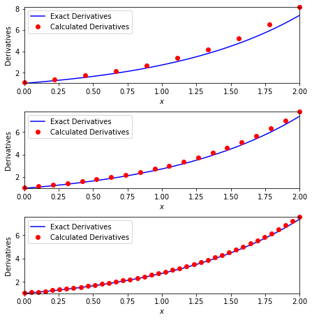
可以观察到我们用前向差分得到的导数随着 $h$ 的减小,逐渐靠近真实值。
6. 小结:舍入误差 vs. 离散化误差
我们通过下面这个例子来分析和对比这两个误差。
例子 6:对比两个误差
继续例子 4 中的函数 $f(x) = \mathrm{e} ^x$ 和它的导数 $f'(x) = \mathrm{e} ^x$。取 $x=1$,分别用前面提到的三种有限微分方法求出数值导数,并与真实值比较计算出相对误差。
这里我们来观察,当 $h$ 取不同值($10^{-1}$ 至 $10^{-15}$)的时候,相对误差的变化情况。
import matplotlib.pyplot as plt
import numpy as np

def ForwardDiff(fx, x, h=0.001):
    # Forward difference
    return (fx(x+h) - fx(x))/h

def CentralDiff(fx, x, h=0.001):
    # Central difference
    return (fx(x+h) - fx(x-h))/h*0.5

def FivePointsDiff(fx, x, h=0.001):
    # Five points difference
    return (-fx(x+2*h) + 8*fx(x+h) - 8*fx(x-h) + fx(x-2*h)) / (12.0*h)

# choose h from 0.1 to 10^-t, t>=2
t = 15
hx = 10**np.linspace(-1,-t, 30)

# The exact derivative at x=1
x0 = 1
fprimExact = np.exp(1)

# Numerical derivative using the three methods
fprimF = ForwardDiff(np.exp, x0, hx)
fprimC = CentralDiff(np.exp, x0, hx)
fprim5 = FivePointsDiff(np.exp, x0, hx)

# Relative error
felF = abs(fprimExact - fprimF)/abs(fprimExact)
felC = abs(fprimExact - fprimC)/abs(fprimExact)
fel5 = abs(fprimExact - fprim5)/abs(fprimExact)

# Plot
fig, ax = plt.subplots(1)
ax.loglog(hx, felF)
ax.loglog(hx, felC)
ax.loglog(hx, fel5)
ax.autoscale(enable=True, axis='x', tight=True)
ax.set_xlabel(r'Step length $h$')
ax.set_ylabel('Relative error')
ax.legend(['Forward difference',
    'Central difference', 'Five points difference'])
<matplotlib.legend.Legend at 0x12066aad0>
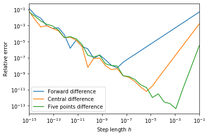
这是一个非常有趣的结果,我们发现
- 这三种方法的相对误差,随着 $h$ 的不同,呈现出两种不同的特性。
- 当 $h$ 较大时(右半侧),误差曲线相对规则,是由离散化误差主导的。
- 当 $h$ 较小时(左半侧),误差曲线波动较大,是由舍入误差主导。
注:舍入误差主导且随着 $h$ 减小而增大的主要原因是:
- 当 $h$ 较小时,有限差分法的分子上相近的数相减会造成类似例子 2 和 3 中的舍入误差。
- 由于这个例子中的 $f(x)$ 在 $e$ 附近,因此这个误差应为 $10^{-16}$ 左右。它除以较小的 $h$ 时,就会被相应的放大,当 $h$ 越小,这个舍入误差越大。
因此,当我们使用上述方法时,需要注意,尽可能取 $h$ 在误差曲线的右半侧,这样我们对于误差才有完全的控制。
同时,我们也观察到,对于越是高阶的差分(如五点差分),它的离散化误差随 $h$ 的下降速率越大,但也越早到达舍入误差的区域。因此,当我们遇到类似问题上,应选择合适阶数的有限差分方法,并根据它的特性选择适合的 $h$ 值。并不一定是越高阶的方法越好, $h$ 越小越好。
本文中所用函数的完整代码见 github。